The techniques of equivalence partitioning and boundary value analysis are often applied to specific situations or inputs. However, if different combinations of inputs result in different actions being taken, this can be more difficult to show using equivalence partitioning and boundary value analysis, which tend to be more focused on the user interface. The other two specification-based software testing techniques, decision tables and state transition testing are more focused on business logic or business rules.
A decision table is a good way to deal with combinations of things (e.g. inputs). This technique is sometimes also referred to as a ’cause-effect’ table. The reason for this is that there is an associated logic diagramming technique called ’cause-effect graphing’ which was sometimes used to help derive the decision table (Myers describes this as a combinatorial logic network [Myers, 1979]). However, most people find it more useful just to use the table described in [Copeland, 2003].
Decision tables provide a systematic way of stating complex business rules, which is useful for developers as well as for testers.
Decision tables can be used in test design whether or not they are used in specifications, as they help testers explore the effects of combinations of different inputs and other software states that must correctly implement business rules.
It helps the developers to do a better job can also lead to better relationships with them. Testing combinations can be a challenge, as the number of combinations can often be huge. Testing all combinations may be impractical if not impossible. We have to be satisfied with testing just a small subset of combinations but making the choice of which combinations to test and which to leave out is also important. If you do not have a systematic way of selecting combinations, an arbitrary subset will be used and this may well result in an ineffective test effort.
How to Use decision tables for test designing?
The first task is to identify a suitable function or subsystem which reacts according to a combination of inputs or events. The system should not contain too many inputs otherwise the number of combinations will become unmanageable. It is better to deal with large numbers of conditions by dividing them into subsets and dealing with the subsets one at a time. Once you have identified the aspects that need to be combined, then you put them into a table listing all the combinations of True and False for each of the aspects.
Let us consider an example of a loan application, where you can enter the amount of the monthly repayment or the number of years you want to take to pay it back (the term of the loan). If you enter both, the system will make a compromise between the two if they conflict. The two conditions are the loan amount and the term, so we put them in a table (see Table 4.2).
TABLE 4.2 Empty decision table:
Conditions Rule 1 Rule 2 Rule 3 Rule 4
Repayment amount has
been entered:
Term of loan has been
Entered:
Next we will identify all of the combinations of True and False (see Table 4.3). With two conditions, each of which can be True or False, we will have four combinations (two to the power of the number of things to be combined). Note that if we have three things to combine, we will have eight combinations, with four things, there are 16, etc. This is why it is good to tackle small sets of combinations at a time. In order to keep track of which combinations we have, we will alternate True and False on the bottom row, put two Trues and then two Falses on the row above the bottom row, etc., so the top row will have all Trues and then all Falses (and this principle applies to all such tables).
TABLE 4.3 Decision table with input combinations:
Conditions Rule 1 Rule 2 Rule 3 Rule 4
Repayment amount has T T F F
been entered:
Term of loan has been T F T F
entered:
In the next step we will now identify the correct outcome for each combination (see Table 4.4). In this example, we can enter one or both of the two fields. Each combination is sometimes referred to as a rule.
TABLE 4.4 Decision table with combinations and outcomes:
Conditions Rule 1 Rule 2 Rule 3 Rule 4
Repayment amount has T T F F
been entered:
Term of loan has been T F T F
entered:
Actions/Outcomes
Process loan amount: Y Y
Process term: Y Y
At this point, we may realize that we hadn’t thought about what happens if the customer doesn’t enter anything in either of the two fields. The table has highlighted a combination that was not mentioned in the specification for this example. We could assume that this combination should result in an error message, so we need to add another action (see Table 4.5). This highlights the strength of this technique to discover omissions and ambiguities in specifications. It is not unusual for some combinations to be omitted from specifications; therefore this is also a valuable technique to use when reviewing the test basis.
TABLE 4 . 5 Decision table with additional outcomes:
Conditions Rule 1 Rule 2 Rule 3 Rule 4
Repayment amount has T T F F
been entered:
Term of loan has been T F T F
entered:
Actions/Outcomes
Process loan amount: Y Y
Process term: Y Y
Error message: Y
Now, we make slight change in this example, so that the customer is not allowed to enter both repayment and term. Now the outcome of our table will change, because there should also be an error message if both are entered, so it will look like Table 4.6.
TABLE 4 . 6 Decision table with changed outcomes:
Conditions Rule 1 Rule 2 Rule 3 Rule 4
Repayment amount has T T F F
been entered:
Term of loan has been T F T F
entered:
Actions/Outcomes
Process loan amount: Y
Process term: Y
Error message: Y Y
You might notice now that there is only one ‘Yes’ in each column, i.e. our actions are mutually exclusive – only one action occurs for each combination of conditions. We could represent this in a different way by listing the actions in the cell of one row, as shown in Table 4.7. Note that if more than one action results from any of the combinations, then it would be better to show them as separate rows rather than combining them into one row.
TABLE 4.7 Decision table with outcomes in one row:
Conditions Rule 1 Rule 2 Rule 3 Rule 4
Repayment amount has T T F F
been entered:
Term of loan has been T F T F
entered:
Actions/Outcomes:
Result: Error Process loan Process Error
message amount term message
The final step of this technique is to write test cases to exercise each of the four rules in our table.
Credit card example:
Let’s take another example. If you are a new customer and you want to open a credit card account then there are three conditions first you will get a 15% discount on all your purchases today, second if you are an existing customer and you hold a loyalty card, you get a 10% discount and third if you have a coupon, you can get 20% off today (but it can’t be used with the ‘new customer’ discount). Discount amounts are added, if applicable. This is shown in Table 4.8.
TABLE 4.8 Decision table for credit card example
Decision table for credit card example
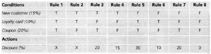
In Table 4.8, the conditions and actions are listed in the left hand column. All the other columns in the decision table each represent a separate rule, one for each combination of conditions. We may choose to test each rule/combination and if there are only a few this will usually be the case. However, if the number of rules/combinations is large we are more likely to sample them by selecting a rich subset for testing.
Now let’s see the decision table for credit card shown above:
Note that we have put X for the discount for two of the columns (Rules 1 and 2) – this means that this combination should not occur. You cannot be both a new customer and also holding a loyalty card as per the conditions mentioned above. Hence there should be an error message stating this.
We have made an assumption in Rule 3. Since the coupon has a greater discount than the new customer discount, we assume that the customer will choose 20% rather than 15%. We cannot add them, since the coupon cannot be used with the ‘new customer’ discount as stated in the condition above. The 20% action is an assumption on our part, and we should check that this assumption (and any other assumptions that we make) is correct, by asking the person who wrote the specification or the users.
For Rule 5, however, we can add the discounts; since both the coupon and the loyalty card discount should apply (that’s our assumption).
Rules 4, 6 and 7 have only one type of discount and Rule 8 has no discount, so 0%.
If we are applying this technique thoroughly, we would have one test for each column or rule of our decision table. The advantage of doing this is that we may test a combination of things that otherwise we might not have tested and that could find a defect. However, if we have a lot of combinations, it may not be possible or sensible to test every combination. If we are time-constrained, we may not have time to test all combinations. Don’t just assume that all combinations need to be tested. It is always better to prioritize and test the most important combinations. Having the full table helps us to decide which combinations we should test and which not to test this time. In the example above all the conditions are binary, i.e. they have only two possible values: True or False (or we can say Yes or No).